Network meta-analysis: application and practice using R software

Sung Ryul Shim; Seong-Jang Kim; Jonghoo Lee; Gerta Rücker

doi:10.4178/epih.e2019013

Articles

Page Path: HOME > Epidemiol Health > Volume 41; 2019 > Article

Methods Network meta-analysis: application and practice using R software: Sung Ryul Shim^1,2, Seong-Jang Kim^3,4, Jonghoo Lee⁵, Gerta Rücker⁶; Epidemiol Health 2019;41:e2019013.
DOI: https://doi.org/10.4178/epih.e2019013
Published online: April 8, 2019

¹Department of Preventive Medicine, Korea University College of Medicine, Seoul, Korea

²Urological Biomedicine Research Institute, Soonchunhyang University Hospital, Seoul, Korea

³Department of Nuclear Medicine, Pusan National University Yangsan Hospital, Pusan National University School of Medicine, Yangsan, Korea

⁴BioMedical Research Institute for Convergence of Biomedical Science and Technology, Pusan National University Yangsan Hospital, Yangsan, Korea

⁵Department of Internal Medicine, Jeju National University Hospital, Jeju National University School of Medicine, Jeju, Korea

⁶Institute of Medical Biometry and Statistics, Faculty of Medicine and Medical Center, University of Freiburg, Freiburg, Germany

Correspondence: Sung Ryul Shim Department of Preventive Medicine, Korea University College of Medicine, 145 Anam-ro, Seongbuk-gu, Seoul 02841, Korea E-mail: sungryul.shim@gmail.com

• Received: March 14, 2019 • Accepted: April 8, 2019

This is an open-access article distributed under the terms of the Creative Commons Attribution License (http://creativecommons.org/licenses/by/4.0/), which permits unrestricted use, distribution, and reproduction in any medium, provided the original work is properly cited.

32,014 Views
1,527 Download
174 Web of Science
155 Crossref
189 Scopus

Full Article

Download PDF

Abstract
INTRODUCTION
STATISTICAL APPROACH OF NETWORK META-ANALYSIS
BAYESIAN NMA USING R "gemtc" PACKAGE
COMPARISON OF NMA RESULTS: BAYESIAN VS. FREQUENTIST METHOD AND R VS. STATA SOFTWARE
CONCLUSION
SUPPLEMENTARY MATERIALS
NOTES
ACKNOWLEDGEMENTS
REFERENCES

Abstract

The objective of this study is to describe the general approaches to network meta-analysis that are available for quantitative data synthesis using R software. We conducted a network meta-analysis using two approaches: Bayesian and frequentist methods. The corresponding R packages were “gemtc” for the Bayesian approach and “netmeta” for the frequentist approach. In estimating a network meta-analysis model using a Bayesian framework, the “rjags” package is a common tool. “rjags” implements Markov chain Monte Carlo simulation with a graphical output. The estimated overall effect sizes, test for heterogeneity, moderator effects, and publication bias were reported using R software. The authors focus on two flexible models, Bayesian and frequentist, to determine overall effect sizes in network meta-analysis. This study focused on the practical methods of network meta-analysis rather than theoretical concepts, making the material easy to understand for Korean researchers who did not major in statistics. The authors hope that this study will help many Korean researchers to perform network meta-analyses and conduct related research more easily with R software.
Keywords: Network meta-analysis, Multiple treatments meta-analysis, Mixed treatment comparison, Consistency, Transitivity, Bayes’ theorem

INTRODUCTION

Network meta-analysis (NMA), also called multiple treatment meta-analysis, or mixed treatment comparison, aims to synthesize the effect sizes of several studies that evaluate multiple interventions or treatments [1-4].

In the conventional pairwise meta-analysis, the researchers collect studies that evaluate the same treatment, create pairs of the treatment group and control group, and directly calculate the effect size (direct treatment comparison). However, NMA can calculate the effect size between treatment groups through indirect treatment comparison, even if there is no direct comparison study, or if the treatments are different between the treatment groups.

In the present study, the previous meta-analysis studies [1-3] are reviewed using R software. This study focuses on the technical implementation of Bayesian NMA and frequentist NMA using R. Thus, it requires understanding of the direct treatment comparison (which is the basic principle of NMA), indirect treatment comparison through common comparators, and mixed treatment comparison that combines direct and indirect treatment comparisons, as well as prior learning about the assumptions of NMA. These concepts are described in previous studies [1-3].

The NMA methods are largely divided into Bayesian methods and frequentist methods. These two statistical methods have different basic concepts for approaching the statistical model, but produce the same results if the sample size is large.; The Bayesian method calculates the posterior probability that the research hypothesis is true by adding the information given in the present data (likelihood) to previously known information (prior probability or external information). Therefore, it can be said that the Bayesian method is a probabilistic approach, where the probability that the research hypothesis is true can be changed depending on the prior information [1,2].; In contrast, the frequentist method calculates the probability of significance (in general, p-value is 0.05) or the 95% confidence interval (CI) for rejecting or accepting the research hypothesis when the present data is repeated infinitely based on a general statistical theory. Therefore, the frequentist method is unrelated to external information, and the probability that the research hypothesis is true within the present data (likelihood) is already specified, and it only determines whether or not to accept or reject it based on the significance level [1,2].
Bayesian method: The frequentist method considers the parameters that represent the characteristics of the population as fixed constants and infers them using the likelihood of the given data. However, the Bayesian method expresses the degree of uncertainty with a probability model by applying the probability concept to the parameters.; The most important characteristics of the Bayesian method are as follows.; First, it can use prior information. For example, if the prior information of the parameter of interest exists (from previous research or empirical knowledge of the relevant disease), updated posterior information can be inferred by adding the prior information to the present data. This is much more logical and persuasive than the frequentist assumption that the given data is repeated infinitely.; Second, it is free from the large sample assumption, because the parameters are considered as random variables. For example, the frequentist meta-analysis assumes that the overall effect size follows a normal distribution. In other words, the normality assumption of the normal distribution is satisfactory for a large sample, but most meta-analysis studies have a small number of studies, and the overall effect size may be biased. However, the Bayesian method calculates the posterior information by adding prior information to the likelihood of the given data, and the parameters are probability concepts that can change continuously. Thus, it is free from the effect of a large sample [2,5].; When the parameter of interest is θ, the prior information follows the prior distribution P(θ). When event χ is observed in the present study, the likelihood is P(χ|θ).; Therefore, the posterior distribution function of the updated parameter of interest θ, becomes P(θ|χ) by multiplying the prior distribution by the likelihood function, as follows:; In the conditional probability equation (1), P(χ) is a fixed constant and omitted in general; thus, the equation can be expressed as (2), where ∝ means “proportional”. If the sample size is large, the influence of prior information P(θ) is weak, and a similar result as that of the frequentist method is obtained. However, if the sample size is small and the amount of prior information P(θ) is large, the posterior distribution will produce a different result. Therefore, the Bayesian method generally shows the sensitivity analysis according to the prior distribution.; Prior distributions are largely divided into subjective and objective. The subjective prior distribution can reflect the results of previous studies or empirical knowledge of the disease. In contrast, the objective prior distribution is an informationless prior distribution, which must be objectively quantified and input to the prior distribution.; The prior distribution that is the same as the posterior distribution is called a conjugate prior distribution. The posterior distribution is inferred using the normal distribution if the parameter is average, beta distribution if it is a ratio, or inverse gamma distribution if it is variance.; For non-conjugate prior distribution, it is not easy to integrate the probability of the derived posterior distribution, because it is not generally used in statistical models [5].; For distributions commonly used in statistics, the area under the distribution curve can be simply obtained with an integral formula. However, with the Bayesian method, it is difficult to calculate it if the posterior distribution does not follow a commonly used distribution. In this case, the Markov chain Monte Carlo (MCMC) simulation can be used to calculate it reversely. In this study, we will briefly review the concepts of MCMC as a tool for Bayesian inference.; Markov chain; In a Markov chain, the probability that a random variable will reach a certain state depends only on the previous state.; Therefore, the next state is determined by the likelihood ratio of the current state and the transition probability, which is prior information. In the initial simulation, the value of the next state is significantly different from the current state, but when this calculation is repeated, the difference becomes very small at a certain time, and it reaches a stable steady-state distribution.; To summarize again, the Markov chain uses an algorithm that calculates the probability of the next state knowing the current state and transition probability, and there is no change in the probability after a certain number of repeated calculations.; Monte Carlo simulation; In Figure 1, let us assume that we want to find the area of a 1/4 circle with a radius of 1. This can be calculated easily by 1/4 * πr²=1/4*3.142*1², which is 0.7855.; In Monte Carlo simulation, a square around the 1/4 circle is created, and many dots are printed randomly in the square. Then, the desired area can be determined by comparing the number of dots within a distance of 1 from the center of the circle with the total number of dots. For example, if a simulation is performed in which a total of 100 dots is printed, the number of dots within a distance of 1 from the center of the circle will be approximately 78.55. Certainly, the difference between the simulated values and the measured values will decrease as the number of simulations increases.; In the fixed effect model, which only considers the within-study variations, the average and variance of the standard normal distribution are input to the prior distribution as follows:; where T_i is the actual observation effect of the ith study, and v_i is the variance of the ith study. Here, θ is the true value of the treatment effect and a common effect size to be inferred by the fixed effect model.; In the random effect model, which considers both within-study and between-study variations, the total average treatment effect of the population (μ) and the between-study variance (τ²) are input to the prior distribution. In turn, μ follows a hyperprior distribution, which is a normal distribution with μ₀ as mean and η₀² as variance, and τ² follows a hyperprior distribution with p as mean and q as variance. These parameters μ₀, η₀², p, and q of the prior distributions μ and τ² are hyperparameters.; In this way, in the random effect model, the treatments effect of each study are connected by the hyperprior distributions from θ_i to θ_k. 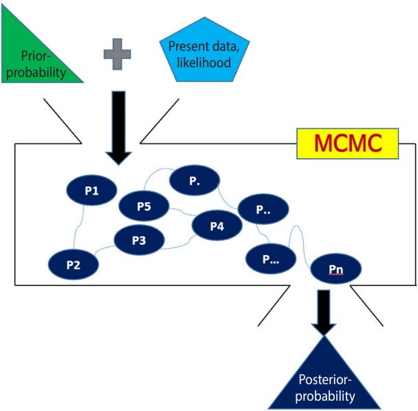Thus, it is no longer an independent model but a hierarchical model [5].; With Figure 2, the Bayesian method can be summarized as follows.; First, a prior distribution (prior probability) is selected. For a conjugate prior distribution, normal distribution, beta distribution, and inverse gamma distribution are generally used.; Second, the likelihood is calculated from the present data and a Bayesian hierarchical model is created – in NMA, the likelihood is mainly expressed as the treatment effect θ.; Third, the prior distribution and likelihood are input to the MCMC simulation, and a distribution that best converges the posterior distribution is set. The probability of stable distribution and the area under the posterior distribution function can be determined through the MCMC simulation.; Lastly, statistical reasoning for the treatment effect is performed with the determined posterior distribution. Therefore, the Bayesian NMA can analyze the posterior distribution even if it is not a standard distribution generally used in statistics.
Frequentist method: The frequentist method is not related to external information, and the probability that the research hypothesis is true within the present data (likelihood) is already specified (test for a p-value of 0.05 or a 95% CI). Thus, it only determines whether to accept or reject the research hypothesis by the significance level.; The following shows the design by treatment interaction model for inconsistency:; where A denotes the reference treatment, J denotes the comparative treatment (J=B,C,…), d denotes the study design, and i denotes the ith study in the dth study design.; The design by treatment interaction model is a frequentist NMA model that considers both heterogeneity between studies and inconsistency between study designs [4].; Here, ydiAJ represents the effect size of J treatment in contrast to the A reference treatment in the ith study of the dth study design, considering heterogeneity between studies and inconsistency between study designs. It is called mean difference, log risk-ratio, or log odds ratio (OR). Next, δ^AJ represents the treatment contrast as a primary index of interest, and the effect size of J treatment in contrast to the A reference treatment. Then, βdiAJ represents the heterogeneity between studies in the same d study design. It is the same as calculating the interstudy variation τ² with a random effect model in pairwise meta-analysis. Then, ωdAJ represents inconsistency. he loop inconsistency is based on Lu & Ades [6], and the design inconsistency was approached through meta-regression analysis of the difference between study designs. Obviously, in the consistency model that satisfies the consistency assumption, ωdAJ =0 for all study designs (d) and contrast treatment (J).; εdiAJ is a within-study error. Generally, it is assumed normal distribution.

Figure 3 shows the flowchart for using the R package "gemtc" for NMA using the Bayesian method. When coding the data first, you must set the variable names in accordance with the relevant function. The process is as follows: network setup -> select a network model (fixed or random) -> select the MCMC convergence optimal model -> statistical reasoning in the final model (Figure 3).; There are two R packages for NMA: “gemtc” for Bayesian NMA and “netmeta” for frequentist NMA. Before starting the analysis, you must install the packages with the following commands. For a more detailed explanation, you can refer to the detailed code, data, and references for each package [7].; · install.packages(“netmeta”); · install.packages(“gemtc”); When running Bayesian NMA, the MCMC simulation is used, and the application required for this is Just Another Gibbs Sampler; Gibbs Sampler is a representative method of MCMC (JAGS). You can download the latest version 4.0 or higher from Google and install it. In addition, you must install the “rjags” package to use JAGS in R as follows:; · install.packages(“rjags”); We mark R commands with a dot (‘· ’) in front of them, to distinguish them from the main text. When long commands are extended to the next line, there is no dot at the beginning of the next line. Thus, when you enter the command in the R software, you must type them without the dot (‘· ’) in front of them.
Data coding and loading: First, load the “gemtc” package to perform Bayesian NMA.; · library(gemtc); Next, load the binary example file from the working directory into the memory of R with the following command. Thus, you should save Supplementary Material 1 as “bin_dn.csv” in the specified working folder.; ·data_b_bin=read.csv(“bin_dn.csv”, header=TRUE); This loaded file is saved as “data_b_bin” in the R memory.; The “gemtc” package has many sub-functions. Among them, the “mtc.network” function can be run only if the data function name is a specific name. In the binary data, it must be “study,” “responders,” “sampleSize,” or “treatment.” In this example, the variable name is different; thus, you must change the variable name with the “colnames” command as follows:; · colnames(data_b_bin) <- c(“study”, “responders”, “sampleSize”, “treatment”); “colnames” specifies the variable name (column), and you must sequentially enter the variable names of data_b_bin data.
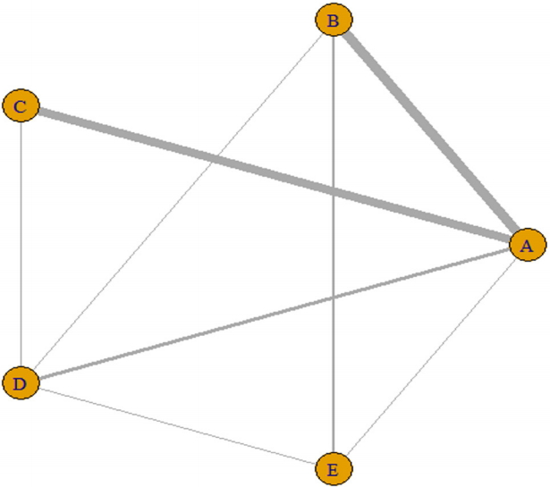
Network setup: For a network analysis of the prepared “data_b_bin” data, you must set up the network using the “mtc.network” function as follows:; · network_b_bin <- mtc.network(data.ab=data_b_bin, description=“Bayesian NMA binary data”); The “mtc.network” function performs network setup with the previously set “data_b_bin” and declares it as “network_b_bin”.; · plot(network_b_bin); The plot function graphically shows the direct comparison between the treatment groups comprising the network (Figure 4). The thickness of the edge for connecting nodes means the amount of data.; · summary(network_b_bin); You can see the overall status of network setup. You can also see the number of 2-arm or 3-arm studies and number of responses to individual treatment. Thus, it numerically describes the above network plot.
Network model: Once the network setup is completed, you must set a network model of fixed effect model or random effect model. Although it is generally recommended to select a random effect model considering the between-study variation, this study will explain with a fixed effect model for convenience.; · model_b_bin_fe <- mtc.model(network_b_bin, linearModel=‘fixed’, n.chain=4); With the “mtc.model” function, you can load the network setup data “network_b_bin” and set the fixed effect model and random effect model as “model_b_bin_fe”. “n.chain” indicates the number of chains to be performed in the following MCMC simulation.
Markov chain Monte Carlo (MCMC) simulation and convergence diagnosis: Once the network model is set up, you can perform a MCMC simulation. The overall process is to set and run an appropriate number of simulations, and then check whether the results converge.; First, an example of the fixed effect model will be explained.; · mcmc_b_bin_fe <- mtc.run(model_b_bin_fe, n.adapt=5000, n.iter=10000, thin=20); In the “mtc.run” function, enter the name of the fixed effect model that has been set. “n.adapt=5000” means to discard no.1-5,000 of the iterations. This is called burn-in, which is to remove a certain part of the beginning of the created random numbers to exclude the effect of the initial values of the algorithm. “n.iter=10000” means to perform 10,000 simulations and “thin=20” means to extract every 20th value.; To summarize the above explanation, the first to 5,000th data are discarded (to reduce the effect of initial values in simulation), simulations are performed 10,000 times with 5,001st to 15,000th values, and every 20th value is extracted (e.g., 5,020, 5,040….).; In the Bayesian analysis, prior distribution considering multichain is input to determine the posterior distribution. The multichain simulation is performed by setting multiple initial values for the prior parameter of prior distribution, that is, the hyperparameter d (e.g., 4 values of -1, 0, 1, and 2). Therefore, because every 20th data are extracted among 10,000 simulations, 500 data points are extracted in each chain.; You can see a more detailed explanation by using the summary command:; · summary(mcmc_b_bin_fe); To verify if the MCMC simulation converged well, you can check the following items in combination.; MCMC error; A smaller MCMC error indicates a higher accuracy, which means a good convergence. Therefore, a sufficient sample size should be achieved by performing many simulations and the burn-in process to remove the effect of initial values, and the data extraction interval “thin” should be adjusted appropriately.; Deviance information criterion; The deviance information criterion (DIC) is expressed as DIC=D¯+pD, where D¯ is the sum of residual deviances and pD is an estimated value of the parameter. 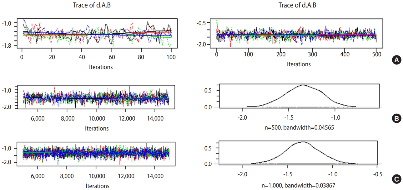Thus, the DIC considers both the fitness and complexity of the model, and the smaller the DIC is, the better the model.; Trace plot and density plot; If the trace plot (a graph visually showing the simulation result) has no specific pattern and the chains are entangled, it is considered that the convergence is good. The density plot is a posterior distribution (posterior density function) and if the shapes are significantly different for the same number of simulations, it means the data did not converge well.; Figure 5A is the case when 100 and 500 were input as the total number of iterations with no burn-in. In the first 100 iterations (Figure 5A left), the four chains have severe variations and are not even, but at approximately 500th iteration (Figure 5A right), the graph becomes even, with no specific pattern. Therefore, it is desirable to perform at least 500 simulations for each channel. For burn-in to exclude the effect of initial values, 1-100th data points must be discarded without question because they are too uneven, and the number of discarded values must be at least 500. In this example, the values were discarded for up to 5,000 times to minimize the effect of the algorithm.; In Figure 5B, when the simulations are performed 10,000 times with an extraction interval “thin” of 20, 500 data points are extracted from each channel. If 10 is input to thin (Figure 5C), 1,000 values are extracted per channel, which increases the sample size and results in a more even distribution of the trace plot. Furthermore, 1,000 samples of post density function were selected because it looks more similar to the normal distribution.; The finally selected model performed burn-in for 5,000 values and 10,000 simulations, and extracted every 10th data point for 1,000 samples per channel.; · mcmc_b_bin_fe <- mtc.run(model_b_bin_fe, n.adapt=5000, n.iter=10000, thin=10); Compared to the extraction interval thin of 20, the total sample size increased and the MCMC standard error of the treatment group AB decreased from 0.004 to 0.003, thus increasing the accuracy. However, the DIC decreased from 56.24 to 56.63, which is practically insignificant.; Gelman-Rubin statistics and plot; · gelman.diag(mcmc_b_bin_fe); · gelman.plot(mcmc_b_bin_fe); The “gelman.diag” command displays the Gelman-Rubin statistics on the console, and the “gelman.plot” command draws the Gelman-Rubin plot. As the number of simulations increases, it approaches 1, and the variations must be stabilized so that it can be said to have converged well.; For MCMC simulation, a model that converges best should be selected by adjusting the number of chains appropriate for multichain, the number of data for removal of initial effect (burn-in), the number of iterations, and the extraction interval (thin).; For the fixed effect model of this example, 4 chains, 5,000 burnins, 10,000 iterations, and an interval of 10 were selected, to sufficiently remove the effect of initial values, increase the iterations and extraction interval, and minimize the MCMC error and DIC variation with almost no variations and stability of various plots.; However, you should adjust the iterations appropriately because it can take significant time depending on the computer specifications.; Burn-in 5,000, iteration 10,000, thin 10; · mcmc_b_bin_fe <- mtc.run(model_b_bin_fe, n.adapt=5000, n.iter=10000, thin=10); · plot(mcmc_b_bin_fe); · summary(mcmc_b_bin_fe); · gelman.diag(mcmc_b_bin_fe); · gelman.plot(mcmc_b_bin_fe); Consistency test in the assumptions of NMA is a critical tool that determines the applicability of NMA results.; · nodesplit_b_bin_fe <- mtc.nodesplit(network_b_bin, linearModel=‘fixed’, n.adapt=5000, n.iter=10000, thin=10); · plot(nodesplit_b_bin_fe); · plot(summary(nodesplit_b_bin_fe)); The fixed effect model “nodesplit_b_bin_fe” is created for consistency test by entering the network set-up data in the “mtc.nodesplit” function. The MCMC simulation is also performed.; The variations between treatments and the consistency test results of all individual treatments can be easily seen. As a result of the consistency test, the p-value of treatments E versus D was 0.043, indicating inconsistency. However, no statistical significance was observed in all the other treatments. 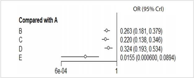Therefore, it is desirable to set up a random effect model for a more robust analysis.; Forest plot allows graphical comparison of the effect sizes by treatment group through NMA.; · forest(relative.effect(mcmc_b_bin_fe, t1=“A”), digits=3); When you enter the final model through MCMC simulation in the forest function, a forest plot with A reference treatment is created (Figure 6).; The effect size (OR, blood transfusion rate) of every treatment was lower than the placebo, and the 95% credible intervals did not overlap.; In particular, the blood transfusion rate of the combination treatment method (E) was statistically significantly lower compared to those of all the other treatments including single intravenous injection (IV) injection [B, IV(single)], double IV injection [C, IV(double)], and topical application method [D, topical].; One of the most important functions of NMA is that the comparative advantages of treatments can be determined. In other words, the cumulative probability that the top priority to the lowest priority treatments are selected can be calculated.; · ranks_b_bin_fe <- rank.probability(mcmc_b_bin_fe, preferredDirection=-1); · print(ranks_b_bin_fe); Enter the final MCMC model in the “rank.probability” function. Set the “preferredDirection” to ‘-1’ or ‘1’, depending on whether a smaller effect size indicates a better treatment, or vice versa. In this example, it is set to ‘-1’ because an effect size smaller than that of the reference treatment means a better treatment.; As can be seen in the probability table, the best treatment is E (combination) at 99.8%, followed by C (IV double) at 68.2%, B (IV single), D (topical), and A (placebo).
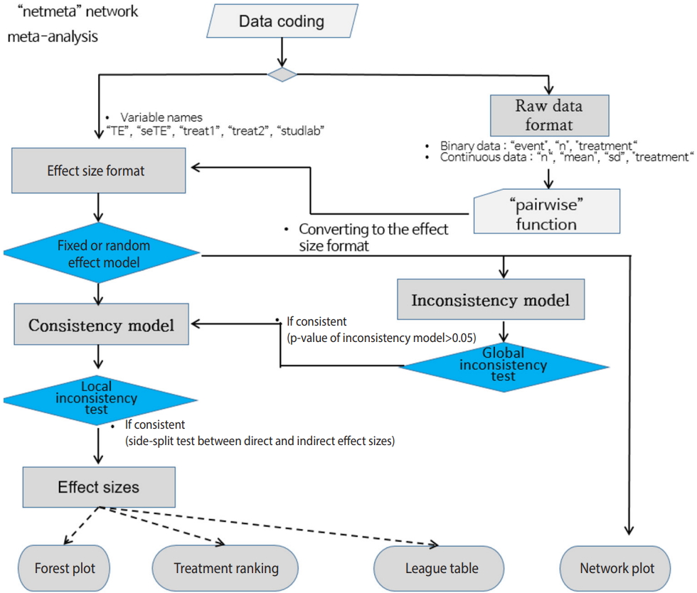
FREQUENTIST NMA USING R “netmeta” PACKAGE: Figure 7 shows the flowchart for using the R package “netmeta” for NMA using the frequentist method. First, you must change the data format to the effect size data format, and set the variable names in accordance with the relevant function. The process is as follows: effect size data format -> select a network model (fixed or random) -> statistical reasoning in the final model.; · library(netmeta); Next, load the binary example file from the working directory into the memory of R with the following command (Supplementary Material 1).; ·data_f_bin=read.csv(“bin_dn.csv”, header=TRUE); The “netmeta” package can be run only if the variable name of the effect size data type is “studlab,” “TE,” “seTE,” “treat1,” or “treat2.” Because the data in this example is raw data, it must be converted to effect size data type, and the variable names must be matched as well.; · data_f_bin <- pairwise(trt, event=d, n=n, studlab=study, data=data_f_bin, sm =“OR” ); Enter the first treatment variable “trt” in the pairwise function, and the other variables are matched: frequency (event=d), sample size (n=n), and study name (studlab=study). Lastly, select whether to use OR or relative risk (RR) data.; If the conversion to the effect size data type has been completed, select the fixed effect model or random effect model for the network model.; · network_f_bin_fe <- netmeta(TE, seTE, treat1, treat2, studlab, data=data_f_bin, sm=“OR”, reference=“A”, comb.fixed=TRUE, comb.random=FALSE); Set the fixed effect model to network_f_bin_fe by loading effect size (TE), standard error (seTE), treatment 1 (treat1), treatment 2 (treat2), study name (studlab), and data_f_bin in the netmeta function.; · tname_f_bin <- c(“Placebo”, “IV(single)”, “IV(double)”, “Topical”, “Combination”); ·netgraph(network_f_bin_fe, labels=tname_f_bin); To enter the treatment name in the network plot, set “tname_f_bin” as the treatment name.; You can enter “network_f_bin_fe” in the “netgraph” function to graphically show a direct comparison between the treatment groups comprising the network. The thickness of the edge for connecting nodes means the amount of data.; Once the network model is set up, you can use “summary” to see the overall summary of the model.; · summary(network_f_bin_fe); The total number of studies is 21, the number of treatments is 5, the number of paired direct comparisons is 25, and the number of study designs is 6 (AB¯, AC¯, AD¯, AE¯, BDE¯, and ABE¯).; Furthermore, the reference variable is A and the effect size is OR.; In this example, the fixed and random effect models have the same effect size because the between-study variance (tau) is zero.; Consistency test in the assumptions of NMA is a critical tool that determines the applicability of NMA results.; This approach calculates the regression coefficient of the inconsistency model for each study design and then tests the linearity of the regression coefficients for all models by using the Wald test. The consistency test was performed for all models in the same way as for the STATA NMA model [4].; · decomp.design(network_f_bin_re); As a result of the consistency test for every model, the p-value was 0.9942. As this supports consistency, which is the null hypothesis, this network model is acceptable.; · print(netsplit(network_f_bin_re), digits=3); Enter the network model in the “netsplit” function and perform a consistency test for each treatment.; In all comparisons of treatments, the p-value was statistically insignificant, showing no inconsistency. Therefore, the consistency model is supported once again.; A forest plot allows a graphical comparison of the effect sizes by treatment group through NMA.; · forest(network_f_bin_fe, ref=“A”, digits=3, xlab=“Odds Ratio”); Enter the set network model and “A” for reference treatment in the forest function.; The effect size (OR, blood transfusion rate) of every treatment was lower than that of the placebo, and the 95% CIs did not overlap.; In particular, the transfusion rate (OR, 0.033; 95% CI, 0.006 to 0.175) of the combination treatment (E) was statistically significantly lower than those of all the other treatments including single IV injection [B, IV (single)] (OR, 0.273; 95% CI, 0.186, to 0.399), double IV injection [C, IV (double)] (OR, 0.229; 95% CI, 0.146, 0.360), and the topical application method [D, topical] (OR, 0.329; 95% CI, 0.197 to 0.550).; One of the most important functions of NMA is that the comparative advantages of treatments can be determined. In other words, the cumulative probability that the top priority to the lowest priority treatments are selected can be calculated.; · ranks_f_bin_fe <- netrank(network_f_bin_fe, small.values=”good”); · print(ranks_f_bin_fe, sort=FALSE); Enter the network model in the “netrank” function. Enter “good” in “small.values” if a smaller effect size indicates a better treatment, or “bad” otherwise.; As can be seen in the probability table, the best treatment is E (combination) at 99.38%, followed by C (IV double) at 65.43%, B (IV single), D (topical), and A (placebo).

COMPARISON OF NMA RESULTS: BAYESIAN VS. FREQUENTIST METHOD AND R VS. STATA SOFTWARE

Table 1 outlines the Bayesian and frequentist NMA. The NMA used in STATA is a design by treatment interaction model based on regression analysis, which considers both heterogeneity between studies and inconsistence between study designs [4]. However, the R “netmeta” package uses an electrical network model, which changed it slightly [8,9].

The Bayesian method also shows similar values between the fixed and random effect models, which is an almost identical result to that of the frequentist method.

CONCLUSION

This paper presented as little statistical theory as possible and focused instead on the actual performance of meta-analysis methods, so that researchers who have not majored in statistics could easily understand it. In other words, this study aimed to provide researchers from different fields an overview of how to adequately use already developed statistical methods in their field of study and interpret the results.

This study compared the Bayesian network meta-analysis using the “gemtc” package and the frequentist network meta-analysis using the “netmeta” package. We found that these two methods produced the same results. Refer to the references for detailed descriptions for continuous data, besides the binary data presented in the examples in this study [2].

We hope that this study will help researchers to perform metaanalysis and conduct related research more easily.

SUPPLEMENTARY MATERIALS

Supplementary materials are available at http://www.e-epih.org/.

epih-41-e2019013-supplementary.pdf

Korean version is available at http://www.e-epih.org/.

epih-41-e2019013-supplementary1.pdf

NOTES

The authors have no conflicts of interest to declare for this study.

ACKNOWLEDGEMENTS

None.

Figure 1.

Monte Carlo simulation.

Figure 2.

Overall concept of the Bayesian approach using a Markov chain Monte Carlo (MCMC) simulation.

Figure 3.

Flow chart of network meta-analysis using the “gemtc” R package. MCMC, Markov chain Monte Carlo; DIC, deviance information criterion.

Figure 4.

Network plot using the “gemtc” package. A: placebo; B: IV (single); C: IV (double); D: topical; E: combination. IV, intravenous injection.

Figure 5.

Trace and density plots: (A) iterations=100 (left) vs. 500 (right); (B) iterations=10,000 & thin=20; (C) iterations=10,000 & thin=10.

Figure 6.

Forest plot_reference A. A: placebo; B: IV (single); C: IV (double); D: topical; E: combination. IV, intravenous; OR, odds ratio; CrI, credible interval.

Figure 7.

Flow chart of network meta-analysis using the “netmeta” R package.

Table 1.

Comparison effect sizes between frequentist and Bayesian method in network meta-analysis

Data type	Treatment	Frequentist approach			Bayesian approach¹
		STATA²	R "nemeta" package		R "gemtc" package
		STATA²	Fixed	Random	Fixed	Random
Binary	Placebo	1.000 (reference)	1.000 (reference)	1.000 (reference)	1.000 (reference)	1.000 (reference)
	IV (single)	0.273 (0.186, 0.399)	0.273 (0.186, 0.399)	0.273 (0.186, 0.399)	0.263 (0.181, 0.379)	0.264 (0.173, 0.399)
	IV (double)	0.229 (0.146, 0.360)	0.229 (0.146, 0.360)	0.229 (0.146, 0.360)	0.220 (0.138, 0.346)	0.220 (0.138, 0.357)
	Topical	0.329 (0.197, 0.550)	0.329 (0.197, 0.550)	0.329 (0.197, 0.550)	0.324 (0.193, 0.534)	0.322 (0.180, 0.551)
	Combination	0.033 (0.006, 0.175)	0.033 (0.006, 0.175)	0.033 (0.006, 0.175)	0.015 (0.001, 0.089)	0.014 (0.000, 0.083)

Values are presented as odds ratio (95% confidence interval).

IV, intravenous injection.

¹ Effect size (95% credible interval).

² Design-by-treatment interaction model.

REFERENCES

1. Hwang SD, Shim SR. Meta-analysis: from forest plot to network meta-analysis. Seoul: Hannarae; 2018. p 180-223 (Korean).
2. Shim SR. Network meta-analysis using R software: Bayesian & frequentist approach. Gwacheon: SDB Lab; 2019. (Korean).
3. Shim S, Yoon BH, Shin IS, Bae JM. Network meta-analysis: application and practice using Stata. Epidemiol Health 2017;39:e2017047.Article PubMed PMC PDF
4. White IR. Network meta-analysis. Stata J 2015;15:951-985.Article
5. Kim DH, Jang EJ, Hwang JS. Meta-analysis using R & WinBUGS. Paju: Free Academy; 2014. p 255-337 (Korean).
6. Lu G, Ades AE. Assessing evidence inconsistency in mixed treatment comparisons. J Am Stat Assoc 2006;101:447-459.Article
7. GitHub. R software “gemtc” & “netmeta” packages. [cited 2018 May 10]. Available from: https://github.com/gertvv/gemtc.
8. Rücker G. Network meta-analysis, electrical networks and graph theory. Res Synth Methods 2012;3:312-324.Article PubMed
9. Rücker G, Schwarzer G. Reduce dimension or reduce weights? Comparing two approaches to multi-arm studies in network meta- analysis. Stat Med 2014;33:4353-4369.Article PubMed

Figure & Data

References

Citations

Citations to this article as recorded by

Effects of game-based digital therapeutics on attention deficit hyperactivity disorder in children and adolescents as assessed by parents or teachers: a systematic review and meta-analysis
SuA Oh, Jina Choi, Doug Hyun Han, EunYoung Kim
European Child & Adolescent Psychiatry.2024; 33(2): 481. CrossRef
Medical Treatment for Peyronie’s Disease: Systematic Review and Network Bayesian Meta-Analysis
Hyun Young Lee, Jong Hyun Pyun, Sung Ryul Shim, Jae Heon Kim
The World Journal of Men's Health.2024; 42(1): 133. CrossRef
Detrusor relaxing agents for neurogenic detrusor overactivity: a systematic review, meta‐analysis and network meta‐analysis
Zhonghan Zhou, Xuesheng Wang, Xunhua Li, Limin Liao
BJU International.2024; 133(1): 25. CrossRef
Efficacy of Various Treatment in Premature Ejaculation: Systematic Review and Network Meta-Analysis
Hyun Young Lee, Jong Hyun Pyun, Sung Ryul Shim, Jae Heon Kim
The World Journal of Men's Health.2024; 42(2): 338. CrossRef
Comparative efficacy and safety of different doses of ponatinib versus other tyrosine kinase inhibitors for the treatment of chronic myeloid leukemia: a systematic review and network meta-analysis
Shan Zhang, Hurong Lai, Huijun Chen, Jingyu Wang, Huaijun Tu, Jian Li
Expert Opinion on Drug Safety.2024; 23(1): 37. CrossRef
Comparing EUS-directed Transgastric ERCP (EDGE) Versus Laparoscopic-Assisted ERCP Versus Enteroscopic ERCP
Manesh K. Gangwani, Muhammad Aziz, Hossein Haghbin, Amna Iqbal, Julia Dillard, Dushyant S. Dahiya, Hassam Ali, Umar Hayat, Sadik Khuder, Wade Lee-Smith, Yusuf Nawras, Faisal Kamal, Sumant Inamdar, Yaseen Alastal, Nirav Thosani, Douglas Adler
Journal of Clinical Gastroenterology.2024; 58(2): 110. CrossRef
Effect of non-pharmacological interventions on pain in preterm infants in the neonatal intensive care unit: a network meta-analysis of randomized controlled trials
Yuwei Weng, Jie Zhang, Zhifang Chen
BMC Pediatrics.2024;[Epub] CrossRef
Denosumab, teriparatide and bisphosphonates for glucocorticoid-induced osteoporosis: a Bayesian network meta-analysis
Liang Dong, Lianghai Jiang, Zhengwei Xu, Xiaobo Zhang
Frontiers in Pharmacology.2024;[Epub] CrossRef
Diagnostic performance of angiography‐derived fractional flow reserve and CT‐derived fractional flow reserve: A systematic review and Bayesian network meta‐analysis
Zhongxiu Chen, Junyan Zhang, Yujia Cai, Hongsen Zhao, Duolao Wang, Chen Li, Yong He
Journal of Evidence-Based Medicine.2024; 17(1): 119. CrossRef
Vascularized Tissue to Reduce Fistula After Salvage Total Laryngectomy: A Network Meta‐analysis
Andrew Williamson, Faizan Shah, Irene Benaran, Vinidh Paleri
The Laryngoscope.2024;[Epub] CrossRef
Endoscopy for acute upper gastrointestinal bleeding: a protocol for systematic review and network meta-analysis of randomized controlled trials
Xiaofang Tang, Lixi Long, Xiaoyun Wang, Yiwu Zhou
International Journal of Surgery Protocols.2024;[Epub] CrossRef
Delving into Human Factors through LSTM by Navigating Environmental Complexity Factors within Use Case Points for Digital Enterprises
Nevena Rankovic, Dragica Rankovic
Journal of Theoretical and Applied Electronic Commerce Research.2024; 19(1): 381. CrossRef
Comparative efficacy and safety of COVID-19 vaccines in phase III trials: a network meta-analysis
Xiaodi Wu, Ke Xu, Ping Zhan, Hongbing Liu, Fang Zhang, Yong Song, Tangfeng Lv
BMC Infectious Diseases.2024;[Epub] CrossRef
Exercise training modalities in prediabetes: a systematic review and network meta-analysis
Hang Zhang, Yuting Guo, Guangshun Hua, Chenyang Guo, Simiao Gong, Min Li, Yan Yang
Frontiers in Endocrinology.2024;[Epub] CrossRef
Single Versus Second Observer vs Artificial Intelligence to Increase the ADENOMA Detection Rate of Colonoscopy—A Network Analysis
Manesh Kumar Gangwani, Hossein Haghbin, Rizwan Ishtiaq, Fariha Hasan, Julia Dillard, Fouad Jabbar, Dushyant Singh Dahiya, Hassam Ali, Shaharyar Salim, Wade Lee-Smith, Amir Sohail, Sumant Inamdar, Muhammad Aziz, Benjamin Hart
Digestive Diseases and Sciences.2024;[Epub] CrossRef
Effects of interventions on smoking cessation: A systematic review and network meta‐analysis
Ying Li, Lei Gao, Yaqing Chao, Jianhua Wang, Tianci Qin, Xiaohua Zhou, Xiaoan Chen, Lingyu Hou, linlin Lu
Addiction Biology.2024;[Epub] CrossRef
Comparative Efficacy of Different Protein Supplements on Muscle Mass, Strength, and Physical Indices of Sarcopenia among Community-Dwelling, Hospitalized or Institutionalized Older Adults Undergoing Resistance Training: A Network Meta-Analysis of Randomiz
Chun-De Liao, Shih-Wei Huang, Hung-Chou Chen, Mao-Hua Huang, Tsan-Hon Liou, Che-Li Lin
Nutrients.2024; 16(7): 941. CrossRef
Safety and efficacy of antioxidant therapy in children and adolescents with attention deficit hyperactivity disorder: A systematic review and network meta-analysis
Peike Zhou, Xiaohui Yu, Tao Song, Xiaoli Hou, Cristina Deppermann Fortes
PLOS ONE.2024; 19(3): e0296926. CrossRef
Comparison of the efficacy and tolerability of different repetitive transcranial magnetic stimulation modalities for post-stroke dysphagia: a systematic review and Bayesian network meta-analysis protocol
Qiang Chen, Mengfan Kan, Xiaoyu Jiang, Huifen Liu, Deqi Zhang, Lin Yuan, Qiling Xu, Hongyan Bi
BMJ Open.2024; 14(4): e080289. CrossRef
Efficacy and safety of tyrosine kinase inhibitors for advanced metastatic thyroid cancer: A systematic review and network meta-analysis of randomized controlled trials
Mingjian Zhao, Ruowen Li, Zhimin Song, Chengxu Miao, Jinghui Lu
Medicine.2024; 103(15): e37655. CrossRef
Chinese herbal medicines for the treatment of depression: a systematic review and network meta-analysis
Chun Dang, Qinxuan Wang, Qian Li, Ying Xiong, Yaoheng Lu
Frontiers in Pharmacology.2024;[Epub] CrossRef
Impact of disease volume on survival efficacy of triplet therapy for metastatic hormone-sensitive prostate cancer: a systematic review, meta-analysis, and network meta-analysis
Akihiro Matsukawa, Pawel Rajwa, Tatsushi Kawada, Kensuke Bekku, Ekaterina Laukhtina, Jakob Klemm, Benjamin Pradere, Keiichiro Mori, Pierre I. Karakiewicz, Takahiro Kimura, Piotr Chlosta, Shahrokh F. Shariat, Takafumi Yanagisawa
International Journal of Clinical Oncology.2024;[Epub] CrossRef
Modified triple Kessler with least risk of elongation among Achilles tendon repair techniques: a systematic review and network meta-analysis of human cadaveric studies
Pedro Diniz, Jácome Pacheco, Ricardo M. Fernandes, Hélder Pereira, Frederico Castelo Ferreira, Gino M. M. J. Kerkhoffs
Knee Surgery, Sports Traumatology, Arthroscopy.2023; 31(5): 1644. CrossRef
Comparative efficacy and safety of prostatic urethral lift vs prostatic artery embolization for benign prostatic hyperplasia: a systematic review and network meta‐analysis
Vanesa Lucas‐Cava, Francisco Miguel Sánchez‐Margallo, Iñigo Insausti‐Gorbea, Fei Sun
BJU International.2023; 131(2): 139. CrossRef
The effectiveness of pressure support ventilation and T‐piece in differing duration among weaning patients: A systematic review and network meta‐analysis
Xiaomei Ye, David Waters, Hong‐Jing Yu
Nursing in Critical Care.2023; 28(1): 120. CrossRef
Motor functional recovery efficacy of scaffolds with bone marrow stem cells in rat spinal cord injury: a Bayesian network meta-analysis
Dong Zhang, Yifeng Sun, Wei Liu
Spinal Cord.2023; 61(2): 93. CrossRef
Efficacy and safety of direct oral anticoagulants for the treatment of cancer-associated venous thromboembolism: A systematic review and Bayesian network meta-analysis
Haoyu Ning, Nana Yang, Yuanyuan Ding, Haokun Chen, Lele Wang, Yuxuan Han, Gang Cheng, Meijuan Zou
Medicina Clínica.2023; 160(6): 245. CrossRef
Association between age and efficacy of combination systemic therapies in patients with metastatic hormone-sensitive prostate cancer: a systematic review and meta-analysis
Pawel Rajwa, Takafumi Yanagisawa, Isabel Heidegger, Fabio Zattoni, Giancarlo Marra, Timo F. W. Soeterik, Roderick C. N. van den Bergh, Massimo Valerio, Francesco Ceci, Claudia V. Kesch, Veeru Kasivisvanathan, Ekaterina Laukhtina, Tatsushi Kawada, Peter Ny
Prostate Cancer and Prostatic Diseases.2023; 26(1): 170. CrossRef
Comparative efficacy and safety of monoamine oxidase type B inhibitors plus channel blockers and monoamine oxidase type B inhibitors as adjuvant therapy to levodopa in the treatment of Parkinson's disease: a network meta‐analysis of randomized controlled
Rui Yan, Huihui Cai, Yusha Cui, Dongning Su, Guoen Cai, Fabin Lin, Tao Feng
European Journal of Neurology.2023; 30(4): 1118. CrossRef
Outcomes of open vs laparoscopic vs robotic vs transanal total mesorectal excision (TME) for rectal cancer: a network meta-analysis
Warren Seow, Nagendra N. Dudi-Venkata, Sergei Bedrikovetski, Hidde M. Kroon, Tarik Sammour
Techniques in Coloproctology.2023; 27(5): 345. CrossRef
Comparison of multiple treatments in the management of transplant-related thrombotic microangiopathy: a network meta-analysis
Jingyi Yang, Xiaoyan Xu, Shiyu Han, Jiaqian Qi, Xueqian Li, Tingting Pan, Rui Zhang, Yue Han
Annals of Hematology.2023; 102(1): 31. CrossRef
Does High-Velocity Resistance Exercise Elicit Greater Physical Function Benefits Than Traditional Resistance Exercise in Older Adults? A Systematic Review and Network Meta-Analysis of 79 Trials
Pedro Lopez, Anderson Rech, Maria Petropoulou, Robert U Newton, Dennis R Taaffe, Daniel A Galvão, Douglas J P Turella, Sandro R Freitas, Régis Radaelli, Lewis A Lipsitz
The Journals of Gerontology: Series A.2023; 78(8): 1471. CrossRef
Efficacy of non-enhanced computer tomography-based radiomics for predicting hematoma expansion: A meta-analysis
Yan-Wei Jiang, Xiong-Jei Xu, Rui Wang, Chun-Mei Chen
Frontiers in Oncology.2023;[Epub] CrossRef
The Efficacy of Different Nerve Blocks on Postoperative Pain and Sequelae in Patients Undergoing Abdominoplasty: A Network Meta-Analysis
Konstantinos Seretis, Nikolaos Bounas
Aesthetic Surgery Journal.2023; 43(5): NP325. CrossRef
Evaluation of Systemic Treatments of Small Intestinal Adenocarcinomas
Tim de Back, Isabelle Nijskens, Pascale Schafrat, Myriam Chalabi, Geert Kazemier, Louis Vermeulen, Dirkje Sommeijer
JAMA Network Open.2023; 6(2): e230631. CrossRef
Based on ARASENS trial: efficacy and safety of darolutamide as an emerging option of endocrinotherapy for metastatic hormone-sensitive prostate cancer—an updated systematic review and network meta-analysis
Maoyang Dou, Hao Liang, Yang Liu, Qiujie Zhang, Ruowen Li, Shouzhen Chen, Benkang Shi
Journal of Cancer Research and Clinical Oncology.2023;[Epub] CrossRef
Different interventions for the treatment of patent ductus arteriosus in children: a protocol for a network meta-analysis
Xin Zhang, Xiao-Dong Hou, Wen-Xin Wang, Kang Yi, Xin-Kuan Wang, Fan Ding, Xin-Xin Li, Tao You
Systematic Reviews.2023;[Epub] CrossRef
Diagnostic value of PET with different radiotracers and MRI for recurrent glioma: a Bayesian network meta-analysis
Tian Xiaoxue, Wang Yinzhong, Qi Meng, Xingru Lu, Junqiang Lei
BMJ Open.2023; 13(3): e062555. CrossRef
Emergency Department Visits in Children Associated with Exposure to Ambient PM1 within Several Hours
Yachen Li, Lifeng Zhu, Yaqi Wang, Ziqing Tang, Yuqian Huang, Yixiang Wang, Jingjing Zhang, Yunquan Zhang
International Journal of Environmental Research and Public Health.2023; 20(6): 4910. CrossRef
Effectiveness and safety of traditional Chinese medicine decoction for diabetic gastroparesis: A network meta-analysis
Yu-Xin Zhang, Yan-Jiao Zhang, Run-Yu Miao, Xin-Yi Fang, Jia-Hua Wei, Yu Wei, Jia-Ran Lin, Jia-Xing Tian
World Journal of Diabetes.2023; 14(3): 313. CrossRef
Efficacy and safety of direct oral anticoagulants for the treatment of cancer-associated venous thromboembolism: A systematic review and Bayesian network meta-analysis
Haoyu Ning, Nana Yang, Yuanyuan Ding, Haokun Chen, Lele Wang, Yuxuan Han, Gang Cheng, Meijuan Zou
Medicina Clínica (English Edition).2023; 160(6): 245. CrossRef
Efficacy of surgical treatment for post-prostatectomy urinary incontinence: a systematic review and network meta-analysis
Jae Joon Park, Yejoon Hong, Allison Kwon, Sung Ryul Shim, Jae Heon Kim
International Journal of Surgery.2023; 109(3): 401. CrossRef
Comparative efficacies of 13 surgical interventions for primary congenital glaucoma in children: a network meta-analysis of randomized clinical trials
Yun Jeong Lee, Ahnul Ha, Donghwee Kang, Sung Ryul Shim, Jin Wook Jeoung, Ki Ho Park, Young Kook Kim
International Journal of Surgery.2023; 109(4): 953. CrossRef
Combination therapy for high-volume versus low-volume metastatic hormone-sensitive prostate cancer: A systematic review and network meta-analysis
Tengteng Jian, Yang Zhan, Ying Yu, Kai Yu, Rui Hu, Jixue Wang, Ji Lu
Frontiers in Pharmacology.2023;[Epub] CrossRef
Efficacy of surgical methods for peri-implantitis: a systematic review and network meta-analysis
Jing Cheng, Liang Chen, Xian Tao, Xiang Qiang, Ruiying Li, Jia Ma, Dong Shi, Zijin Qiu
BMC Oral Health.2023;[Epub] CrossRef
A network meta-analysis on the efficacy and safety of thermal and nonthermal endovenous ablation treatments
Vangelis Bontinis, Alkis Bontinis, Andreas Koutsoumpelis, Angeliki Chorti, Vasileios Rafailidis, Argirios Giannopoulos, Kiriakos Ktenidis
Journal of Vascular Surgery: Venous and Lymphatic Disorders.2023; 11(4): 854. CrossRef
Comparative effects of off-pump and multiple cardiopulmonary bypass strategies in coronary artery bypass grafting surgery: protocol for a systematic review and network meta-analysis
Jia Tan, Sizhe Gao, Yongnan Li, Xuehan Li, Lei Du, Bingyang Ji
BMJ Open.2023; 13(6): e072545. CrossRef
Regional analgesia techniques for lumbar spine surgery: a frequentist network meta-analysis
Boohwi Hong, Sujin Baek, Hyemin Kang, Chahyun Oh, Yumin Jo, Soomin Lee, Seyeon Park
International Journal of Surgery.2023; 109(6): 1728. CrossRef
Comparison of clinical outcomes among total knee arthroplasties using posterior-stabilized, cruciate-retaining, bi-cruciate substituting, bi-cruciate retaining designs: a systematic review and network meta-analysis
Kaibo Sun, Yuangang Wu, Limin Wu, Bin Shen
Chinese Medical Journal.2023; 136(15): 1817. CrossRef
Physical Activity Interventions for Improving Cognitive Functions in Children With Autism Spectrum Disorder: Protocol for a Network Meta-Analysis of Randomized Controlled Trials
Longxi Li, Anni Wang, Qun Fang, Michelle E Moosbrugger
JMIR Research Protocols.2023; 12: e40383. CrossRef
Bayesian estimation and prediction for network meta-analysis with contrast-based approach
Hisashi Noma
The International Journal of Biostatistics.2023;[Epub] CrossRef
Comparison of the efficacy and safety of first-line treatments for of advanced EGFR mutation-positive non-small-cell lung cancer in Asian populations: a systematic review and network meta-analysis
Wei Chen, Julian Miao, Ying Wang, Wenzhong Xing, Xiumei Xu, Rui Wu
Frontiers in Pharmacology.2023;[Epub] CrossRef
GLP-1RAs caused gastrointestinal adverse reactions of drug withdrawal: a system review and network meta-analysis
Ziqi Zhang, Qiling Zhang, Ying Tan, Yu Chen, Xiqiao Zhou, Su Liu, Jiangyi Yu
Frontiers in Endocrinology.2023;[Epub] CrossRef
Network Meta-analysis of Combined Strength and Power Training for Countermovement Jump Height
Maximilian Brandt, Sibylle Beinert, Martin Alfuth
International Journal of Sports Medicine.2023; 44(11): 778. CrossRef
Network meta-analysis of first-line immune checkpoint inhibitor therapy in advanced non-squamous non-small cell lung cancer patients with PD-L1 expression ≥ 50%
Wei Chen, Jiayi Chen, Lin Zhang, Sheng Cheng, Junxian Yu
BMC Cancer.2023;[Epub] CrossRef
A network meta-analysis of therapeutic and prophylactic management of vasospasm on aneurysmal subarachnoid hemorrhage outcomes
Benjamin Chousterman, Brice Leclère, Louis Morisson, Yannick Eude, Etienne Gayat, Alexandre Mebazaa, Raphael Cinotti
Frontiers in Neurology.2023;[Epub] CrossRef
A Systematic Review Network Meta-Analysis and Meta-Regression on Surgical and Endovenous Interventions for the Treatment of Lower Limb Venous Ulcer Disease
Vangelis Bontinis, Kiriakos Ktenidis, Alkis Bontinis, Andreas Koutsoumpelis, Constantine N Antonopoulos, Argirios Giannopoulos, Vasileios Rafailidis, Angeliki Chorti, Andrew W Bradbury
Journal of Endovascular Therapy.2023;[Epub] CrossRef
Comparative efficacy of 24 exercise types on postural instability in adults with Parkinson’s disease: a systematic review and network meta-analysis
Yujia Qian, Xueying Fu, Haoyang Zhang, Yong Yang, Guotuan Wang
BMC Geriatrics.2023;[Epub] CrossRef
Effectiveness and cost-effectiveness of six GLP-1RAs for treatment of Chinese type 2 diabetes mellitus patients that inadequately controlled on metformin: a micro-simulation model
Shuai Yuan, Yingyu Wu
Frontiers in Public Health.2023;[Epub] CrossRef
Optimal type and dose of hypoxic training for improving maximal aerobic capacity in athletes: a systematic review and Bayesian model-based network meta-analysis
Xinmiao Feng, Linlin Zhao, Yonghui Chen, Zihao Wang, Hongyuan Lu, Chuangang Wang
Frontiers in Physiology.2023;[Epub] CrossRef
Efficacy and Safety of Anti-HER2 Targeted Therapy for Metastatic HR-Positive and HER2-Positive Breast Cancer: A Bayesian Network Meta-Analysis
Xian-Meng Wu, Yong-Kang Qian, Hua-Ling Chen, Chen-Hua Hu, Bing-Wei Chen
Current Oncology.2023; 30(9): 8444. CrossRef
Sensitivities evaluation of five radiopharmaceuticals in four common medullary thyroid carcinoma metastatic sites on PET/CT: a network meta-analysis and systematic review
Pengyu Li, Yujie Zhang, Tianfeng Xu, Jingqiang Zhu, Tao Wei, Wanjun Zhao
Nuclear Medicine Communications.2023; 44(12): 1114. CrossRef
What are the most effective exercise, physical activity and dietary interventions to improve body composition in women diagnosed with or at high‐risk of breast cancer? A systematic review and network meta‐analysis
Christine Kudiarasu, Pedro Lopez, Daniel A. Galvão, Robert U. Newton, Dennis R. Taaffe, Lorna Mansell, Brianna Fleay, Christobel Saunders, Caitlin Fox‐Harding, Favil Singh
Cancer.2023; 129(23): 3697. CrossRef
Transdiagnostic MRI markers of psychopathology following traumatic brain injury: a systematic review and network meta-analysis protocol
Alexia Samiotis, Amelia J Hicks, Jennie Ponsford, Gershon Spitz
BMJ Open.2023; 13(9): e072075. CrossRef
The efficacy and adverse events of arsenic trioxide for the patients with myelodysplastic syndrome: a systematic review and component network meta-analysis
Xiaohua Huang, Yuan Liu, Ruixuan Liu, Xiaoqiu Zou, Hongyong Yang
Hematology.2023;[Epub] CrossRef
Different lumbar fusion techniques for lumbar spinal stenosis: a Bayesian network meta-analysis
Wei Li, Haibin Wei, Ran Zhang
BMC Surgery.2023;[Epub] CrossRef
Is moderate resistance training adequate for older adults with sarcopenia? A systematic review and network meta-analysis of RCTs
Yu Chang Chen, Wang-Chun Chen, Chia-Wei Liu, Wei-Yu Huang, ICheng Lu, Chi Wei Lin, Ru Yi Huang, Jung Sheng Chen, Chi Hsien Huang
European Review of Aging and Physical Activity.2023;[Epub] CrossRef
Comparative analysis of surgical interventions for osteonecrosis of the femoral head: a network meta-analysis of randomized controlled trials
Liyou Hu, Xiaolei Deng, Bo Wei, Jian Wang, Decai Hou
Journal of Orthopaedic Surgery and Research.2023;[Epub] CrossRef
Comparison of healing effectiveness of different debridement approaches for diabetic foot ulcers: a network meta-analysis of randomized controlled trials
Peng Ning, Yupu Liu, Jun Kang, Hongyi Cao, Jiaxing Zhang
Frontiers in Public Health.2023;[Epub] CrossRef
Efficacy and safety of ketamine-assisted electroconvulsive therapy in major depressive episode: a systematic review and network meta-analysis
Taeho Greg Rhee, Sung Ryul Shim, Jonah H. Popp, Thomas A. Trikalinos, Robert A. Rosenheck, Charles H. Kellner, Stephen J. Seiner, Randall T. Espinoza, Brent P. Forester, Roger S. McIntyre
Molecular Psychiatry.2023;[Epub] CrossRef
Can exercise promote additional benefits on body composition in patients with obesity after bariatric surgery? A systematic review and meta‐analysis of randomized controlled trials
Giorjines Boppre, Florêncio Diniz‐Sousa, Lucas Veras, José Oliveira, Hélder Fonseca
Obesity Science & Practice.2022; 8(1): 112. CrossRef
Comparison of Systemic Treatments for Metastatic Castration-Resistant Prostate Cancer After Docetaxel Failure: A Systematic Review and Network Meta-analysis
Junru Chen, Yaowen Zhang, Xingming Zhang, Jinge Zhao, Yuchao Ni, Sha Zhu, Ben He, Jindong Dai, Zhipeng Wang, Zilin Wang, Jiayu Liang, Xudong Zhu, Pengfei Shen, Hao Zeng, Guangxi Sun
Frontiers in Pharmacology.2022;[Epub] CrossRef
Different Monoclonal Antibodies in Myasthenia Gravis: A Bayesian Network Meta-Analysis
Zhaoming Song, Jie Zhang, Jiahao Meng, Guannan Jiang, Zeya Yan, Yanbo Yang, Zhouqing Chen, Wanchun You, Zhong Wang, Gang Chen
Frontiers in Pharmacology.2022;[Epub] CrossRef
Effects of curved path walking compared to straight path walking in older adults with cognitive deficits: A systematic review and network meta‐analysis
Han Suk Lee, Sung Ryul Shim, Jun Ho Kim, Mansoo Ko
Physiotherapy Research International.2022;[Epub] CrossRef
Relative Effect of Extracorporeal Shockwave Therapy Alone or in Combination with Noninjective Treatments on Pain and Physical Function in Knee Osteoarthritis: A Network Meta-Analysis of Randomized Controlled Trials
Chun-De Liao, Yu-Yun Huang, Hung-Chou Chen, Tsan-Hon Liou, Che-Li Lin, Shih-Wei Huang
Biomedicines.2022; 10(2): 306. CrossRef
Optimal management of functional anorectal pain: a systematic review and network meta-analysis
Kevin Gerard Byrnes, Shaheel Mohammad Sahebally, Niamh McCawley, John Patrick Burke
European Journal of Gastroenterology & Hepatology.2022; 34(3): 249. CrossRef
Comparative Efficacy of Acupuncture-Related Techniques for Urinary Retention After a Spinal Cord Injury: A Bayesian Network Meta-Analysis
Kelin He, Xinyun Li, Bei Qiu, Linzhen Jin, Ruijie Ma
Frontiers in Neurology.2022;[Epub] CrossRef
Comparative effect of different strategies for the screening of lung cancer: a systematic review and network meta-analysis
Yancong Chen, Zixuan Zhang, Huan Wang, Xuemei Sun, Yali Lin, Irene X. Y. Wu
Journal of Public Health.2022; 30(12): 2937. CrossRef
A comprehensive systematic review and network meta-analysis: the role of anti-angiogenic agents in advanced epithelial ovarian cancer
Aya El Helali, Charlene H. L. Wong, Horace C. W. Choi, Wendy W. L. Chan, Naomi Dickson, Steven W. K. Siu, Karen K. Chan, Hextan Y. S. Ngan, Roger K. C. Ngan, Richard D. Kennedy
Scientific Reports.2022;[Epub] CrossRef
Current Therapies in Patients With Posterior Semicircular Canal BPPV, a Systematic Review and Network Meta-analysis
Daibo Li, Danni Cheng, Wenjie Yang, Ting Chen, Di Zhang, Jianjun Ren, Yu Zhao
Otology & Neurotology.2022; 43(4): 421. CrossRef
Comparable Cardiorenal Benefits of SGLT2 Inhibitors and GLP-1RAs in Asian and White Populations: An Updated Meta-analysis of Results From Randomized Outcome Trials
Huilin Tang, Stephen E. Kimmel, Steven M. Smith, Kenneth Cusi, Weilong Shi, Matthew Gurka, Almut G. Winterstein, Jingchuan Guo
Diabetes Care.2022; 45(4): 1007. CrossRef
Intensification of Systemic Therapy in Addition to Definitive Local Treatment in Nonmetastatic Unfavourable Prostate Cancer: A Systematic Review and Meta-analysis
Pawel Rajwa, Benjamin Pradere, Giorgio Gandaglia, Roderick C.N. van den Bergh, Igor Tsaur, Sung Ryul Shim, Takafumi Yanagisawa, Ekaterina Laukhtina, Keiichiro Mori, Hadi Mostafaei, Fahad Quhal, Piotr Bryniarski, Eva Compérat, Guilhem Roubaud, Christophe M
European Urology.2022; 82(1): 82. CrossRef
Comparison of the Efficacy and Safety of a Doravirine-Based, Three-Drug Regimen in Treatment-Naïve HIV-1 Positive Adults: A Bayesian Network Meta-Analysis
Ke Zhang, Yang Zhang, Jing Zhou, Lulu Xu, Chi Zhou, Guanzhi Chen, Xiaojie Huang
Frontiers in Pharmacology.2022;[Epub] CrossRef
Comparison of the Effectiveness of Various Drug Interventions to Prevent Etomidate-Induced Myoclonus: A Bayesian Network Meta-Analysis
Kang-Da Zhang, Lin-Yu Wang, Dan-Xu Zhang, Zhi-Hua Zhang, Huan-Liang Wang
Frontiers in Medicine.2022;[Epub] CrossRef
Effectiveness of five interventions used for prevention of gestational diabetes
Qiongyao Tang, Ying Zhong, Chenyun Xu, Wangya Li, Haiyan Wang, Yu Hou
Medicine.2022; 101(15): e29126. CrossRef
Efficacy of pelvic floor muscle exercise or therapy with or without duloxetine: a systematic review and network Meta-analysis
Jae Joon Park, Allison Kwon, Tae Il Noh, Yong Nam Gwon, Sung Ryul Shim, Jae Heon Kim
The Aging Male.2022; 25(1): 145. CrossRef
Oral and long‐acting antipsychotics for relapse prevention in schizophrenia‐spectrum disorders: a network meta‐analysis of 92 randomized trials including 22,645 participants
Giovanni Ostuzzi, Federico Bertolini, Federico Tedeschi, Giovanni Vita, Paolo Brambilla, Lorenzo del Fabro, Chiara Gastaldon, Davide Papola, Marianna Purgato, Guido Nosari, Cinzia Del Giovane, Christoph U. Correll, Corrado Barbui
World Psychiatry.2022; 21(2): 295. CrossRef
Does the subepithelial connective tissue graft in conjunction with a coronally advanced flap remain as the gold standard therapy for the treatment of single gingival recession defects? A systematic review and network meta‐analysis
Leandro Chambrone, João Botelho, Vanessa Machado, Paulo Mascarenhas, José João Mendes, Gustavo Avila‐Ortiz
Journal of Periodontology.2022; 93(9): 1336. CrossRef
Cost-effectiveness analysis of donafenib versus lenvatinib for first-line treatment of unresectable or metastatic hepatocellular carcinoma
Rui Meng, Xueke Zhang, Ting Zhou, Mengjie Luo, Yijin Qiu
Expert Review of Pharmacoeconomics & Outcomes Research.2022; 22(7): 1079. CrossRef
Complications and cosmetic outcomes of materials used in cranioplasty following decompressive craniectomy—a systematic review, pairwise meta-analysis, and network meta-analysis
Jakob V. E. Gerstl, Luis F. Rendon, Shane M. Burke, Joanne Doucette, Rania A. Mekary, Timothy R. Smith
Acta Neurochirurgica.2022; 164(12): 3075. CrossRef
Diagnostic Performance of Antigen Rapid Diagnostic Tests, Chest Computed Tomography, and Lung Point-of-Care-Ultrasonography for SARS-CoV-2 Compared with RT-PCR Testing: A Systematic Review and Network Meta-Analysis
Sung Ryul Shim, Seong-Jang Kim, Myunghee Hong, Jonghoo Lee, Min-Gyu Kang, Hyun Wook Han
Diagnostics.2022; 12(6): 1302. CrossRef
Regional analgesia techniques for video-assisted thoracic surgery: a frequentist network meta-analysis
Yumin Jo, Seyeon Park, Chahyun Oh, Yujin Pak, Kuhee Jeong, Sangwon Yun, Chan Noh, Woosuk Chung, Yoon-Hee Kim, Young Kwon Ko, Boohwi Hong
Korean Journal of Anesthesiology.2022; 75(3): 231. CrossRef
Endoscopic Delivery of Polymers Reduces Delayed Bleeding after Gastric Endoscopic Submucosal Dissection: A Systematic Review and Meta-Analysis
Youli Chen, Xinyan Zhao, Dongke Wang, Xinghuang Liu, Jie Chen, Jun Song, Tao Bai, Xiaohua Hou
Polymers.2022; 14(12): 2387. CrossRef
Efficacy and Safety of Various First-Line Therapeutic Strategies for Fetal Tachycardias: A Network Meta-Analysis and Systematic Review
Jiangwei Qin, Zhengrong Deng, Changqing Tang, Yunfan Zhang, Ruolan Hu, Jiawen Li, Yimin Hua, Yifei Li
Frontiers in Pharmacology.2022;[Epub] CrossRef
Hypoglycemic agents and glycemic variability in individuals with type 2 diabetes: A systematic review and network meta-analysis
SuA Oh, Sujata Purja, Hocheol Shin, Minji Kim, Eunyoung Kim
Diabetes and Vascular Disease Research.2022; 19(3): 147916412211068. CrossRef
Comparative Efficacy of Different Repetitive Transcranial Magnetic Stimulation Protocols for Stroke: A Network Meta-Analysis
Yuan Xia, Yuxiang Xu, Yongjie Li, Yue Lu, Zhenyu Wang
Frontiers in Neurology.2022;[Epub] CrossRef
Comparison of Preoperative Imaging Modalities for the Assessment of Malignant Potential of Pancreatic Cystic Lesions
Sang-Woo Lee, Sung Ryul Shim, Shin Young Jeong, Seong-Jang Kim
Clinical Nuclear Medicine.2022; 47(10): 849. CrossRef
Interventions for Improving Body Composition in Men with Prostate Cancer: A Systematic Review and Network Meta-analysis
PEDRO LOPEZ, ROBERT U. NEWTON, DENNIS R. TAAFFE, FAVIL SINGH, PHILIPPA LYONS-WALL, LAURIEN M. BUFFART, COLIN TANG, DICKON HAYNE, DANIEL A. GALVÃO
Medicine & Science in Sports & Exercise.2022; 54(5): 728. CrossRef
Optimal induction chemotherapy regimen for locoregionally advanced nasopharyngeal carcinoma: an update Bayesian network meta-analysis
Qiuji Wu, Shaojie Li, Jia Liu, Yahua Zhong
European Archives of Oto-Rhino-Laryngology.2022; 279(11): 5057. CrossRef
A Network Meta-Analysis of the Dose–Response Effects of Dapagliflozin on Efficacy and Safety in Adults With Type 1 Diabetes
Yinhui Li, Hui Li, Liming Dong, Dandan Lin, Lijuan Xu, Pengwei Lou, Deng Zang, Kai Wang, Li Ma
Frontiers in Endocrinology.2022;[Epub] CrossRef
Addition of Capecitabine to Adjuvant Chemotherapy May be the Most Effective Strategy for Patients With Early-Stage Triple-Negative Breast Cancer: A Network Meta-Analysis of 9 Randomized Controlled Trials
Zhiyang Li, Jiehua Zheng, Zeqi Ji, Lingzhi Chen, Jinyao Wu, Juan Zou, Yiyuan Liu, Weixun Lin, Jiehui Cai, Yaokun Chen, Yexi Chen, Hai Lu
Frontiers in Endocrinology.2022;[Epub] CrossRef
Should We Use Hyperbaric Oxygen for Carbon Monoxide Poisoning Management? A Network Meta-Analysis of Randomized Controlled Trials
Yu-Wan Ho, Ping-Yen Chung, Sen-Kuang Hou, Ming-Long Chang, Yi-No Kang
Healthcare.2022; 10(7): 1311. CrossRef
New technologies promoting active upper limb rehabilitation after stroke: an overview and network meta-analysis
Gauthier EVERARD, Louise DECLERCK, Christine DETREMBLEUR, Sophie LEONARD, Glenn BOWER, Stéphanie DEHEM, Thierry LEJEUNE
European Journal of Physical and Rehabilitation Medicine.2022;[Epub] CrossRef
Continuous Subcutaneous Insulin Infusion (CSII) Combined with Oral Glucose-Lowering Drugs in Type 2 Diabetes: A Systematic Review and Network Meta-Analysis of Randomized, Controlled Trials
Hui Li, Aimin Yang, Shi Zhao, Elaine YK Chow, Mohammad Javanbakht, Yinhui Li, Dandan Lin, Lijuan Xu, Deng Zang, Kai Wang, Li Ma
Pharmaceuticals.2022; 15(8): 953. CrossRef
Evidence-Based Approaches for Determining Effective Target Antigens to Develop Vaccines against Post-Weaning Diarrhea Caused by Enterotoxigenic Escherichia coli in Pigs: A Systematic Review and Network Meta-Analysis
Eurade Ntakiyisumba, Simin Lee, Gayeon Won
Animals.2022; 12(16): 2136. CrossRef
Androgen Receptor Signaling Inhibitors in Addition to Docetaxel with Androgen Deprivation Therapy for Metastatic Hormone-sensitive Prostate Cancer: A Systematic Review and Meta-analysis
Takafumi Yanagisawa, Pawel Rajwa, Constance Thibault, Giorgio Gandaglia, Keiichiro Mori, Tatsushi Kawada, Wataru Fukuokaya, Sung Ryul Shim, Hadi Mostafaei, Reza Sari Motlagh, Fahad Quhal, Ekaterina Laukhtina, Maximilian Pallauf, Benjamin Pradere, Takahiro
European Urology.2022; 82(6): 584. CrossRef
Effects of Different Treatment Regimens on Primary Spontaneous Pneumothorax: A Systematic Review and Network Meta-Analysis
Muredili Muhetaer, Keriman Paerhati, Qingchao Sun, Desheng Li, Liang Zong, Haiping Zhang, Liwei Zhang
Annals of Thoracic and Cardiovascular Surgery.2022; 28(6): 389. CrossRef
Assessment of three types of surgical procedures for supravalvar aortic stenosis: A systematic review and meta-analysis
Lizhi Lv, Xinyue Lang, Simeng Zhang, Cheng Wang, Qiang Wang
Frontiers in Cardiovascular Medicine.2022;[Epub] CrossRef
Comparative efficacy and safety of immunotherapy for patients with advanced or metastatic esophageal squamous cell carcinoma: a systematic review and network Meta-analysis
Tian-Tian Gao, Jia-Hui Shan, Yu-Xian Yang, Ze-Wei Zhang, Shi-Liang Liu, Mian Xi, Meng-Zhong Liu, Lei Zhao
BMC Cancer.2022;[Epub] CrossRef
Optimal Pharmacologic Treatment of Heart Failure With Preserved and Mildly Reduced Ejection Fraction
Boyang Xiang, Ruiqi Zhang, Xiaoguang Wu, Xiang Zhou
JAMA Network Open.2022; 5(9): e2231963. CrossRef
Adjuvant therapy in neonatal sepsis to prevent mortality - A systematic review and network meta-analysis
T. Abiramalatha, V.V. Ramaswamy, T. Bandyopadhyay, S.H. Somanath, N.B. Shaik, V.R. Kallem, A.K. Pullattayil, M. Kaushal
Journal of Neonatal-Perinatal Medicine.2022; 15(4): 699. CrossRef
Efficacy and safety of monotherapy and combination therapy of immune checkpoint inhibitors as first-line treatment for unresectable hepatocellular carcinoma: a systematic review, meta-analysis and network meta-analysis
Qing Lei, Xin Yan, Huimin Zou, Yixuan Jiang, Yunfeng Lai, Carolina Oi Lam Ung, Hao Hu
Discover Oncology.2022;[Epub] CrossRef
Efficacy and evaluation of therapeutic exercises on adults with Parkinson’s disease: a systematic review and network meta-analysis
Yong Yang, Guotuan Wang, Shikun Zhang, Huan Wang, Wensheng Zhou, Feifei Ren, Huimin Liang, Dongdong Wu, Xinying Ji, Makoto Hashimoto, Jianshe Wei
BMC Geriatrics.2022;[Epub] CrossRef
Efficacy of Neurostimulations for Upper Extremity Function Recovery after Stroke: A Systematic Review and Network Meta-Analysis
Tao Xue, Zeya Yan, Jiahao Meng, Wei Wang, Shujun Chen, Xin Wu, Feng Gu, Xinyu Tao, Wenxue Wu, Zhouqing Chen, Yutong Bai, Zhong Wang, Jianguo Zhang
Journal of Clinical Medicine.2022; 11(20): 6162. CrossRef
Effect of Exercise Interventions on Health-Related Quality of Life in Patients with Fibromyalgia Syndrome: A Systematic Review and Network Meta-Analysis
Kang-Da Zhang, Lin-Yu Wang, Zhi-Hua Zhang, Dan-Xu Zhang, Xiao-Wen Lin, Tao Meng, Feng Qi
Journal of Pain Research.2022; Volume 15: 3639. CrossRef
Comparative efficacy of exercise modalities for cardiopulmonary function in hemodialysis patients: A systematic review and network meta-analysis
Wanli Zang, Mingqing Fang, He He, Liang Mu, Xiaoqin Zheng, Heng Shu, Nan Ge, Su Wang
Frontiers in Public Health.2022;[Epub] CrossRef
Association of Glucose-Lowering Drugs With Outcomes in Patients With Diabetes Before Hospitalization for COVID-19
Zheng Zhu, Qingya Zeng, Qinyu Liu, Junping Wen, Gang Chen
JAMA Network Open.2022; 5(12): e2244652. CrossRef
A Meta-Analysis on the Impact of the COVID-19 Pandemic on Cutaneous Melanoma Diagnosis in Europe
Konstantinos Seretis, Nikolaos Bounas, Georgios Gaitanis, Ioannis Bassukas
Cancers.2022; 14(24): 6085. CrossRef
Complementary and alternative therapies for generalized anxiety disorder: A protocol for systematic review and network meta-analysis
Kai Song, Yating Wang, Li Shen, Jinwei Wang, Rong Zhang
Medicine.2022; 101(51): e32401. CrossRef
Comparison the efficacy and safety of different neoadjuvant regimens for resectable and borderline resectable pancreatic cancer: a systematic review and network meta-analysis
Xujia Li, Jinsheng Huang, Chang Jiang, Ping Chen, Qi Quan, Qi Jiang, Shengping Li, Guifang Guo
European Journal of Clinical Pharmacology.2022;[Epub] CrossRef
Effect of liposomal bupivacaine on opioid requirements and length of stay in colorectal enhanced recovery pathways: A systematic review and network meta‐analysis
Kevin Gerard Byrnes, Shaheel Mohammad Sahebally, John Patrick Burke
Colorectal Disease.2021; 23(3): 603. CrossRef
Metaanálisis y comparaciones indirectas. Métodos y paradigma: tratamiento biológico de la psoriasis
L. Puig
Actas Dermo-Sifiliográficas.2021; 112(3): 203. CrossRef
Repetitive transcranial magnetic stimulation for lower extremity motor function in patients with stroke: a systematic review and network meta-analysis
Yun-Juan Xie, Yi Chen, Hui-Xin Tan, Qi-Fan Guo, BensonWui-Man Lau, Qiang Gao
Neural Regeneration Research.2021; 16(6): 1168. CrossRef
Meta-analysis and Indirect Comparisons: on Methods, Paradigms, and Biologic Treatments for Psoriasis
L. Puig
Actas Dermo-Sifiliográficas (English Edition).2021; 112(3): 203. CrossRef
Diagnostic values of F-18 FDG PET or PET/CT, CT, and US for Preoperative Lymph Node Staging in Thyroid Cancer: A Network Meta-Analysis
Keunyoung Kim, Sung-Ryul Shim, Sang-Woo Lee, Seong-Jang Kim
The British Journal of Radiology.2021; 94(1120): 20201076. CrossRef
A Systematic Review and Network Meta-analyses to Assess the Effectiveness of Human Immunodeficiency Virus (HIV) Self-testing Distribution Strategies
Ingrid Eshun-Wilson, Muhammad S Jamil, T Charles Witzel, David V Glidded, Cheryl Johnson, Noelle Le Trouneau, Nathan Ford, Kathleen McGee, Chris Kemp, Stefan Baral, Sheree Schwartz, Elvin H Geng
Clinical Infectious Diseases.2021; 73(4): e1018. CrossRef
Comparison of PECS II and erector spinae plane block for postoperative analgesia following modified radical mastectomy: Bayesian network meta-analysis using a control group
Boohwi Hong, Seunguk Bang, Chahyun Oh, Eunhye Park, Seyeon Park
Journal of Anesthesia.2021; 35(5): 723. CrossRef
Resistance Training Load Effects on Muscle Hypertrophy and Strength Gain: Systematic Review and Network Meta-analysis
PEDRO LOPEZ, RÉGIS RADAELLI, DENNIS R. TAAFFE, ROBERT U. NEWTON, DANIEL A. GALVÃO, GABRIEL S. TRAJANO, JULIANA L. TEODORO, WILLIAM J. KRAEMER, KEIJO HÄKKINEN, RONEI S. PINTO
Medicine & Science in Sports & Exercise.2021; 53(6): 1206. CrossRef
Relative Efficacy of Weight Management, Exercise, and Combined Treatment for Muscle Mass and Physical Sarcopenia Indices in Adults with Overweight or Obesity and Osteoarthritis: A Network Meta-Analysis of Randomized Controlled Trials
Shu-Fen Chu, Tsan-Hon Liou, Hung-Chou Chen, Shih-Wei Huang, Chun-De Liao
Nutrients.2021; 13(6): 1992. CrossRef
Comparative efficacy of glucose‐lowering medications on body weight and blood pressure in patients with type 2 diabetes: A systematic review and network meta‐analysis
Apostolos Tsapas, Thomas Karagiannis, Panagiota Kakotrichi, Ioannis Avgerinos, Chrysanthi Mantsiou, Georgios Tousinas, Apostolos Manolopoulos, Aris Liakos, Konstantinos Malandris, David R. Matthews, Eleni Bekiari
Diabetes, Obesity and Metabolism.2021; 23(9): 2116. CrossRef
Diagnostic Values of 8 Different Imaging Modalities for Preoperative Detection of Axillary Lymph Node Metastasis of Breast Cancer
Keunyoung Kim, Sung-Ryul Shim, Seong-Jang Kim
American Journal of Clinical Oncology.2021; 44(7): 331. CrossRef
Comparison of Antipsychotics for the Treatment of Patients With Delirium and QTc Interval Prolongation: A Clinical Decision Analysis
Ken Kurisu, Kazuhiro Yoshiuchi
Frontiers in Psychiatry.2021;[Epub] CrossRef
Tailored Versus Standard Hydration to Prevent Acute Kidney Injury After Percutaneous Coronary Intervention: Network Meta‐Analysis
Francesco Moroni, Luca Baldetti, Conrad Kabali, Carlo Briguori, Mauro Maioli, Anna Toso, Emmanouil S. Brilakis, Hitinder S. Gurm, Rodrigo Bagur, Lorenzo Azzalini
Journal of the American Heart Association.2021;[Epub] CrossRef
Three-Drug Regimens Containing Integrase Inhibitor Show Good Efficacy and Safety in Treatment-Naive Patients With HIV-1: A Bayesian Analysis
Ke Zhang, Yang Zhang, Xinchao Liu, Aixin Li, Meixia Gao, Jianhua Hou, Chunxiang Guo, Tong Zhang, Hao Wu, Guanzhi Chen, Xiaojie Huang
Frontiers in Pharmacology.2021;[Epub] CrossRef
Postoperative oral drug regimen to control the inflammatory complications in mandibular third molar surgery: protocol for a systematic review and network meta-analysis
Glaciele Maria de Souza, Rafael Alvim Magesty, Ighor Andrade Fernandes, Késsia Nara Andrade Sales, Endi Lanza Galvão, Saulo Gabriel Moreira Falci
JBI Evidence Synthesis.2021; 19(8): 2024. CrossRef
Research and scholarly methods: Meta‐analysis
William L. Baker, Diana M. Sobieraj
JACCP: JOURNAL OF THE AMERICAN COLLEGE OF CLINICAL PHARMACY.2021; 4(9): 1170. CrossRef
Concepts and emerging issues of network meta-analysis
EunJin Ahn, Hyun Kang
Korean Journal of Anesthesiology.2021; 74(5): 371. CrossRef
Effectiveness comparisons of various therapies for FIGO stage IB2/IIA2 cervical cancer: a Bayesian network meta-analysis
Jing Cheng, Beibei Liu, Biao Wang, Xicui Long, Zhihong Li, Ruili Chen, Ruiting Wu, Lin Xu
BMC Cancer.2021;[Epub] CrossRef
Effects of Anti-Diabetic Drugs on Fracture Risk: A Systematic Review and Network Meta-Analysis
Yu-Sheng Zhang, Yan-Dan Zheng, Yan Yuan, Shi-Chun Chen, Bao-Cheng Xie
Frontiers in Endocrinology.2021;[Epub] CrossRef
Effect of Acupuncture on Movement Function in Patients with Parkinson’s Disease: Network Meta-Analysis of Randomized Controlled Trials
Miri Kwon, Moon Joo Cheong, Jungtae Leem, Tae-hun Kim
Healthcare.2021; 9(11): 1502. CrossRef
Comparative efficacy of mitochondrial agents for bipolar disorder during depressive episodes: a network meta-analysis using frequentist and Bayesian approaches
Rituparna Maiti, Archana Mishra, Biswa Ranjan Mishra, Monalisa Jena
Psychopharmacology.2021; 238(12): 3347. CrossRef
Network meta-analysis for clinicians
Alexey A. Bogdanov, Andrey A. Bogdanov
Journal of Modern Oncology.2021; 23(3): 418. CrossRef
Which Probiotic Is the Most Effective for Treating Acute Diarrhea in Children? A Bayesian Network Meta-Analysis of Randomized Controlled Trials
Zengbin Li, Guixian Zhu, Chao Li, Hao Lai, Xin Liu, Lei Zhang
Nutrients.2021; 13(12): 4319. CrossRef
Outcomes Associated with First-Line anti-PD-1/ PD-L1 agents vs. Sunitinib in Patients with Sarcomatoid Renal Cell Carcinoma: A Systematic Review and Meta-Analysis
Buonerba, Dolce, Iaccarino, Scafuri, Verde, Costabile, Pagliuca, Morra, Riccio, Ribera, De Placido, Romeo, Crocetto, Longo, Imbimbo, De Placido, Lorenzo
Cancers.2020; 12(2): 408. CrossRef
A simulation study to compare different estimation approaches for network meta-analysis and corresponding methods to evaluate the consistency assumption
Corinna Kiefer, Sibylle Sturtz, Ralf Bender
BMC Medical Research Methodology.2020;[Epub] CrossRef
Comparison of 5 Different PET Radiopharmaceuticals for the Detection of Recurrent Medullary Thyroid Carcinoma
Sang-Woo Lee, Sung Ryul Shim, Shin Young Jeong, Seong-Jang Kim
Clinical Nuclear Medicine.2020; 45(5): 341. CrossRef
Determining optimal strategies for primary prevention of cardiovascular disease: systematic review, cost-effectiveness review and network meta-analysis protocol
Olalekan A. Uthman, Lena Al-Khudairy, Chidozie U. Nduka, Rachel Court, Hema Mistry, G . J. Melendez-Torres, Sian Taylor-Phillips, Aileen Clarke
Systematic Reviews.2020;[Epub] CrossRef
Systematic review and sequential network meta‐analysis on the efficacy of periodontal regenerative therapies
Shang‐Jie Tsai, Yu‐Wei Ding, Ming‐Chieh Shih, Yu‐Kang Tu
Journal of Clinical Periodontology.2020; 47(9): 1108. CrossRef
Perspective of the comparative effectiveness of non-pharmacologic managements on postpartum hemorrhage using a network meta-analysis
Kyung Ju Lee, Kwan Hong, Hari Hwang, Hijeong Choi, Sangho Sohn
Obstetrics & Gynecology Science.2020; 63(5): 605. CrossRef
Efficacy of noninvasive respiratory support modes for primary respiratory support in preterm neonates with respiratory distress syndrome: Systematic review and network meta‐analysis
Viraraghavan Vadakkencherry Ramaswamy, Kiran More, Charles Christoph Roehr, Prathik Bandiya, Sushma Nangia
Pediatric Pulmonology.2020; 55(11): 2940. CrossRef
Optimal treatment strategy of fremanezumab in migraine prevention: a systematic review with network meta-analysis of randomized clinical trials
I-Hsin Huang, Po-Chien Wu, Ya-Han Lee, Yi-No Kang
Scientific Reports.2020;[Epub] CrossRef
Comparison of different transcatheter interventions for treatment of mitral regurgitation
Bowen Zhang, Muyang Li, Yingying Kang, Lina Xing, Yu Zhang
Medicine.2020; 99(50): e23623. CrossRef
Bayesian network analysis of open, laparoscopic, and robot-assisted radical cystectomy for bladder cancer
Lin Dong, Yu Qin, Lu Ya, Cao Liang, Hu Tinghui, He Pinlin, Yang Jin, Wang Youliang, Cui Shu, Wu Tao
Medicine.2020; 99(52): e23645. CrossRef
Immune-checkpoint inhibitor plus chemotherapy versus conventional chemotherapy for treatment of recurrent or metastatic head and neck squamous cell carcinoma: a systematic review and network meta-analysis
Zhe Jin, Bin Zhang, Lu Zhang, Wenhui Huang, Xiaokai Mo, Qiuyin Chen, Fei Wang, Zhuozhi Chen, Minmin Li, Shuixing Zhang
Therapeutic Advances in Medical Oncology.2020; 12: 175883592098371. CrossRef
Safety and efficacy characteristics of oral drugs in patients with premature ejaculation: a Bayesian network meta-analysis of randomized controlled trials
Zhiqiang Qin, Yi Wang, Jundong Zhu, Kai Zhu, Ran Li, Lei Zhang, Xianghu Meng, Jiadong Xia, Wei Wang, Chao Qin, Wei Zhang, Ninghong Song, Zengjun Wang
International Journal of Impotence Research.2019; 31(5): 356. CrossRef